Portfolio Optimization with Python
A basic introduction to portfolio optimization, focusing on asset allocation and maximizing the Sharpe ratio, presented from a programmer's perspective.
- Published on
- Last updated on:

Table of Contents
Modern Portfolio Theory (MPT)
Modern Portfolio Theory (MPT) is a practical approach that guides the selection of investments to maximize overall returns while managing risk effectively. By employing a mathematical framework, MPT facilitates the construction of portfolios that optimize the balance between expected returns and acceptable levels of risk. The goal is to achieve the highest expected return possible for a given level of risk through a well-diversified portfolio.
The theory was pioneered by Harry Markowitz in 1952 and earned him the Nobel. The very common assumption among people is that you need to take higher risks to get higher returns; lower-risk investments will give you lower returns. But Markowitz showed that you can get higher returns with lower risk by diversifying your portfolio.
Efficient frontier
The efficient frontier is the set of optimal portfolios that offer the highest expected return for a defined level of risk or the lowest risk for a given level of expected return. Portfolios that lie below the efficient frontier are suboptimal because they do not provide enough return for the level of risk.
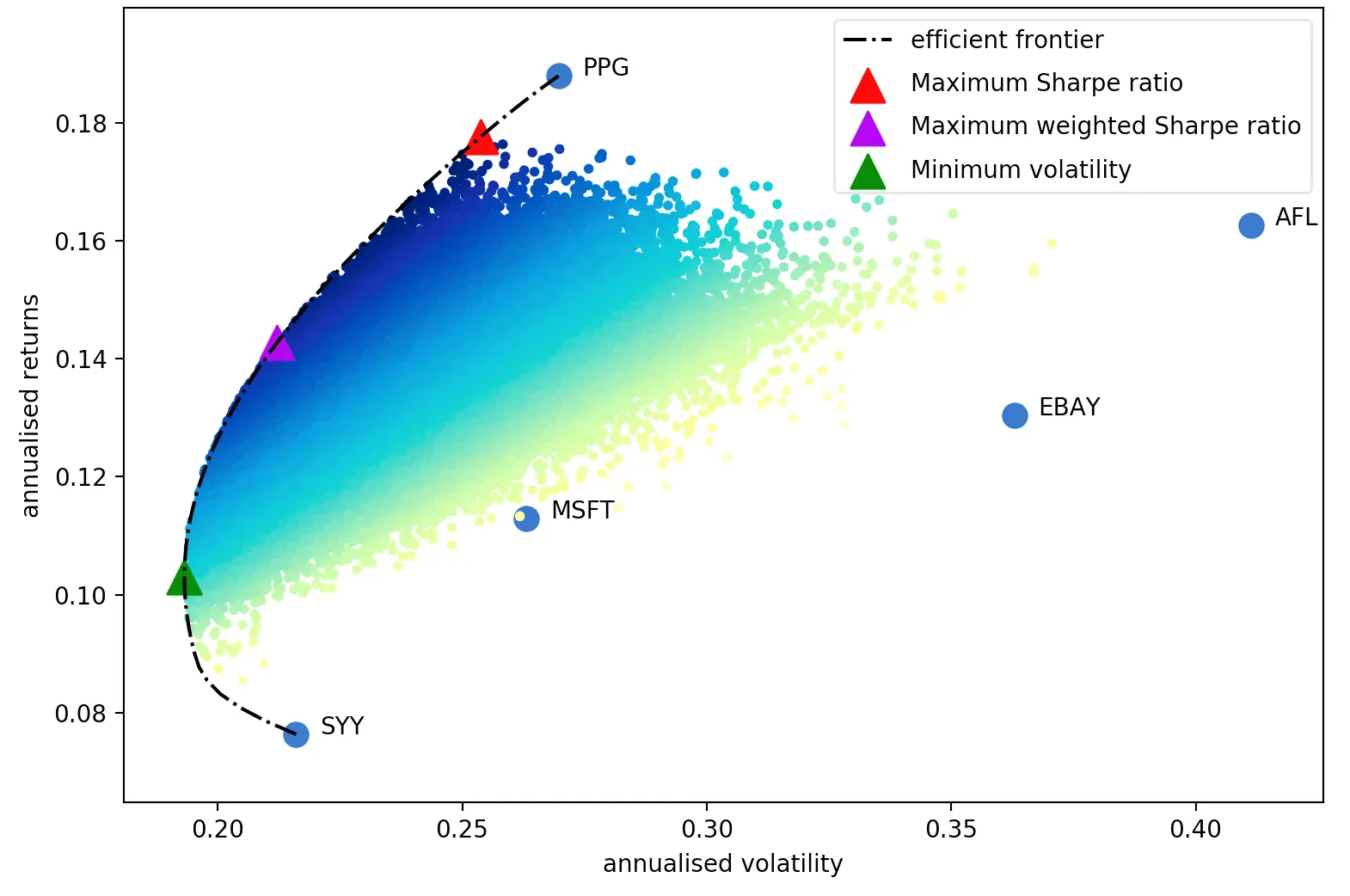
A risk-averse investor will select investments located at the left end of the efficient frontier, which consists of securities with lower risk but lower returns. On the other hand, a risk-seeking investor will choose investments located at the right end of the efficient frontier, which consists of securities expected to have high potential returns along with a high degree of risk.
Sharpe ratio
The sharpe ratio is used by market experts and investors to calculate whether an investment is worth taking the associated risks. Technically, the sharpe ratio measures the average return of an investment that exceeds the risk-free rate per unit of deviation. Therefore, when comparing two different financial assets, the one with a higher sharpe ratio is considered better and more worthy of investment.
Sharpe ratio formula
Sharpe ratio = (Rp - Rf) / σp
Rpis the expected return of the portfolioRfis the risk-free rateσpis the standard deviation of the portfolio
The risk-free rate is the theoretical rate of return of a risk-free investment. e.g., government bonds. If you are investing in government bonds, you are taking no risk (at least in theory), and you are guaranteed to get a return at a fixed rate.
Finding the optimal portfolio with Python
After the brief introduction to modern portfolio theory and glossary, let’s try to find our optimal portfolio with Python. There are a lot of libraries available for portfolio optimization. I will use PyPortfolioOpt, so let’s start with installing it. This is a convex optimization problem, so you can also use SciPy or CVXPY to solve it.
Installing PyPortfolioOpt
pip install PyPortfolioOpt
Installing Pandas
pip install pandas
Installing Finance API
We need to retrieve historical data of the assets we want to include in our portfolio. I’ve developed an app for retrieving historical data of the assets from Yahoo Finance and TEFAS. You can find the click-to-run executable or the source code of the app here.
After downloading the app, if you want to compile from the source code, you can run the following command:
go run main.go serve
If Golang is not installed on your machine, you can download the binary from the releases.
When you run the app, it will start a web server on port 8090. We will use its HTTP API to retrieve historical data of the assets.
Retrieving historical data of the assets
The API I’ve developed can return prices in CSV format, and we can use them directly in Pandas. To make an API call, we can use a function like the following:
import pandas as pd
API_URL = 'http://localhost:8090'
def get_historical_prices(symbol, start_date, end_date):
url = f'{API_URL}/api/yahoo/symbol/{symbol}?startDate={start_date}&endDate={end_date}&format=csv¤cy=TRY'
df = pd.read_csv(url, parse_dates=['Date'])
return df
Now let's define the assets we want to include in our portfolio. And set the start and end dates.
symbols = ["THYAO.IS", "ISMEN.IS", "TTRAK.IS", "TUPRS.IS", "SISE.IS", "EREGL.IS"]
start_date = "2013-10-20"
end_date = "2023-10-20"
By default, the API returns the prices in separate row-oriented CSV files for each symbol. Before using the data with PyPortfolioOpt, we need to convert the data to a column-oriented format for storing the prices of each symbol in a single CSV file.
combined_prices = pd.DataFrame(columns=["Date"] + symbols)

for symbol in symbols:
    prices_df = get_historical_prices(symbol, start_date, end_date)
    prices_df = prices_df[["Date", "Close"]]  # Keep only Date and Close columns
    prices_df = prices_df.rename(columns={"Close": symbol})  # Rename Close column to symbol
    combined_prices = combined_prices.merge(prices_df, how="outer", on="Date")

# After the transpose, we will have _x and _y suffixes for each symbol
# We will remove the _x suffixes because they do not contain any data
# _y suffixes will be kept because they contain the prices
combined_prices = combined_prices.loc[:, ~combined_prices.columns.str.endswith("_x")]

# The API returns prices from the most recent to the oldest
# We will reverse the order to be able to use the data with PyPortfolioOpt
combined_prices = combined_prices.iloc[::-1]

combined_prices.to_csv("combined_prices.csv", index=False)
combined_prices.csv will look like the following.
Date,THYAO.IS_y,ISMEN.IS_y,TTRAK.IS_y,TUPRS.IS_y,SISE.IS_y,EREGL.IS_y
2013-10-21,8.24,0.28773,34.133331,6.271428,2.136561,2.59
2013-10-22,8.36,0.28773,33.866665,6.3,2.122596,2.69
2013-10-23,8.16,0.28773,33.866665,6.457142,2.094668,2.63
2013-10-24,8.34,0.29187,34.533333,6.671428,2.087685,2.64
2013-10-25,8.28,0.29394,34.933334,6.728571,2.10165,2.65
2013-10-28,8.26,0.29601,34.933334,6.857142,2.122596,2.71
2013-10-29,8.26,0.29601,34.933334,6.857142,2.122596,2.71
2013-10-30,8.0,0.30015,35.866665,6.714285,2.10165,2.73
2013-10-31,7.82,0.29808,35.200001,6.471428,2.052774,2.77
2013-11-01,7.92,0.29808,34.666664,6.428571,2.045792,2.75
2013-11-04,7.86,0.30222,33.599998,6.471428,2.003899,2.67
Using PyPortfolioOpt to find the optimal portfolio
After preparing the historical price dataset, we can start using PyPortfolioOpt to find the optimal weights of the assets in our portfolio.
PyPortfolioOpt provides various methods for optimising the portfolio. We will use the max_sharpe method to find the optimal weights when we want to maximise the sharpe ratio.
from pypfopt import EfficientFrontier
from pypfopt import risk_models
from pypfopt import expected_returns

df = pd.read_csv("combined_prices.csv", parse_dates=True, index_col="Date")

# Calculate expected returns and sample covariance
mu = expected_returns.mean_historical_return(df)
S = risk_models.sample_cov(df)

# Optimize for maximal sharpe ratio
ef = EfficientFrontier(mu, S)
raw_weights = ef.max_sharpe()
cleaned_weights = ef.clean_weights()
ef.save_weights_to_file("weights.csv")
print(cleaned_weights)
ef.portfolio_performance(verbose=True)
The output will look like the following:
OrderedDict([('THYAO.IS_y', 0.0063), ('ISMEN.IS_y', 0.64027), ('TTRAK.IS_y', 0.11433), ('TUPRS.IS_y', 0.11282), ('SISE.IS_y', 0.07483), ('EREGL.IS_y', 0.05145)])
Expected annual return: 52.7%
Annual volatility: 27.5%
Sharpe Ratio: 1.85
The results above show that we can get a 52.7% annual return with 27.5% annual volatility.
Backtesting the optimal portfolio
We used the last 10 years of historical data to find the optimal portfolio. We can backtest the optimal portfolio against an equally weighted portfolio and see the results.
Let's compare two scenarios:
- We gave equal weights to all assets in our portfolio a year ago and held them for a year.
- We used the optimal weights we found with
PyPortfolioOpta year ago and held them for a year.start_dateis2013-10-20end_dateis2022-10-20
Equally weighted portfolio
There are six assets in our portfolio. So we will give 1/6 weight to each asset. We can simply calculate the returns of each stock separately and then calculate the average of them.

Optimized portfolio
Results with the new data (we assumed that the last year's data is the new data and was not available when we were optimizing the portfolio).

OrderedDict([('THYAO.IS_y', 0.00784), ('ISMEN.IS_y', 0.60541), ('TTRAK.IS_y', 0.0), ('TUPRS.IS_y', 0.07336), ('SISE.IS_y', 0.16481), ('EREGL.IS_y', 0.14859)])
Expected annual return: 38.9%
Annual volatility: 23.6%
Sharpe Ratio: 1.56
As you can see in the weights above, the optimal portfolio does not include all symbols of the initial portfolio. Optimization algorithm eliminated TTRAK.IS.
Code
import pandas as pd

data = pd.read_csv('combined_prices.csv')

# Filter data for rows since 2022-10-20
start_date = '2022-10-20'
filtered_data = data[data['Date'] >= start_date]

# Calculate return percentage for each stock
return_percentages = {}
for column in filtered_data.columns[1:]:
    initial_price = filtered_data[column].iloc[0]
    current_price = filtered_data[column].iloc[-1]
    return_percentage = ((current_price - initial_price) / initial_price) * 100
    return_percentages[column] = return_percentage

# Display the return percentage for each stock
for stock, percentage in return_percentages.items():
    print(f"Return percentage of {stock}: {round(percentage, 2)}%")

# Calculate average return
average_return = sum(return_percentages.values()) / len(return_percentages)
print(f"Average return: {round(average_return, 2)}%")

# Calculate average return with optimized weights
weights = {
    'THYAO.IS_y': 0.00784,
    'ISMEN.IS_y': 0.60541,
    'TTRAK.IS_y': 0.0,
    'TUPRS.IS_y': 0.07336,
    'SISE.IS_y': 0.16481,
    'EREGL.IS_y': 0.14859
}

weighted_returns = []

for stock, percentage in return_percentages.items():
    weighted_returns.append(percentage * weights[stock])

print(f"Average return with optimized weights: {round(sum(weighted_returns), 2)}%")
Results
Return percentage of THYAO.IS_y: 115.65%
Return percentage of ISMEN.IS_y: 410.04%
Return percentage of TTRAK.IS_y: 382.59%
Return percentage of TUPRS.IS_y: 153.61%
Return percentage of SISE.IS_y: 61.83%
Return percentage of EREGL.IS_y: 32.31%
Average return: 192.67%
Average return with optimized weights: 275.41%

Conclusion
As we can see from the results, investing in the stock market can yield significant returns. The average return was 192.67% with an equally weighted portfolio showcases the potential for growth. However, by optimising the portfolio with carefully selected weights, we were able to attain an impressive average return of 275.41%. This highlights the importance of a strategic portfolio. allocation and the potential benefits it can bring to investors. But please keep in mind that we used past data to find the optimal weights, but we cannot guarantee that the future returns of the stocks will be the same or similar.
Also, it is important to note that portfolio optimization is a dynamic process. that requires monitoring and periodic adjustments to adapt to changing markets conditions. This is called rebalancing and should be done at least once a year.
Disclaimer
This article is for educational purposes only. It should not be considered financial advice. You should consult with a financial advisor or other professional to determine what may be best for your individual needs. I do not make any guarantee or other promise as to any results that may be obtained from using my content.
Resources
- https://www.investopedia.com/terms/m/modernportfoliotheory.asp (Date of access: 21.10.2023)
- https://www.investopedia.com/terms/e/efficientfrontier.asp (Date of access: 21.10.2023)